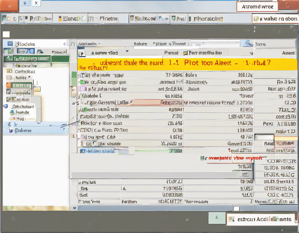
Introduction
Microsoft Excel is a powerful tool that is widely used for data analysis and organization. One of its most useful features is the Pivot Table, which allows users to summarize and analyze large amounts of data with ease. However, many users face difficulty in finding the Pivot Table Insert option within Excel. In this comprehensive guide, we will walk you through the steps to locate this essential feature and make the most of it for your data analysis needs.
Locating the Pivot Table Insert Option
The Pivot Table Insert option in Excel can be found in the “Insert” tab on the Excel ribbon. Here are the detailed steps to locate this option:
-
Open Excel: Launch Microsoft Excel on your computer.
-
Open your Workbook: Open the Excel workbook that contains the data you want to analyze with a Pivot Table.
-
Select your Data: Click on any cell within the range of data you want to analyze. Alternatively, you can select the entire dataset by clicking and dragging over it.
-
Navigate to the Insert Tab: Look at the top menu and click on the “Insert” tab. This tab is where you will find various tools and functions for inserting different elements into your Excel worksheet.
-
Locate the Pivot Table Icon: Within the Insert tab, you will find the “Pivot Table” icon. It is represented by a spreadsheet with a small pivot table icon on the top left corner. Click on this icon to open the Pivot Table creation window.
-
Create your Pivot Table: In the Pivot Table creation window, you can choose the location for your Pivot Table (either a new worksheet or an existing one) and customize the layout and design according to your preferences.
-
Drag and Drop Fields: Once you have created your Pivot Table, you can start dragging and dropping fields from the Field List into the Rows, Columns, Values, or Filters area to analyze your data in various ways.
Why Use Pivot Tables in Excel?
Pivot Tables in Excel are invaluable tools for data analysis due to the following reasons:
- Summarize Data: Pivot Tables allow you to summarize large datasets into compact, understandable formats.
- Visualize Data: They help in converting raw data into visual formats such as charts for better understanding.
- Filter and Sort: Pivot Tables enable you to filter and sort data easily to focus on specific information.
- Perform Calculations: You can perform calculations like sum, average, count, etc., on your dataset within Pivot Tables.
- Dynamic Reports: Pivot Tables create dynamic reports that can be updated with new data with a simple refresh.
Tips for Using Pivot Tables Effectively
To make the most out of Pivot Tables in Excel, consider the following tips:
- Organize your Data: Ensure your data is clean, organized, and in a tabular format before creating a Pivot Table.
- Use Descriptive Headers: Provide clear and concise headers for your columns to ease field selection in the Pivot Table.
- Refresh Data Regularly: If your data source is updated frequently, remember to refresh your Pivot Table to reflect the changes.
- Experiment with Different Layouts: Try different layouts and arrangements of fields within the Pivot Table to find the most insightful view of your data.
- Apply Filters and Sorts: Utilize filters and sorts to focus on specific data points and analyze them in detail.
- Learn Keyboard Shortcuts: Familiarize yourself with keyboard shortcuts for quick navigation and manipulation of Pivot Tables.
Frequently Asked Questions (FAQs)
- What is a Pivot Table in Excel?
-
A Pivot Table is a feature in Excel that allows you to summarize and analyze large datasets with ease by rearranging and aggregating data as per your requirements.
-
Where is the Pivot Table Field List located in Excel?
-
The Pivot Table Field List usually appears on the right side of the Excel window when you create or select a Pivot Table. You can hide or show it using the Field List button in the Pivot Table Analyze or Options tab.
-
Can I create multiple Pivot Tables from the same data in Excel?
-
Yes, you can create multiple Pivot Tables from the same dataset in Excel by selecting different ranges of data or by duplicating an existing Pivot Table.
-
How can I customize the design of my Pivot Table in Excel?
-
You can customize the design of your Pivot Table by changing the layout, styles, and formatting options available under the Pivot Table Design tab once you have created your Pivot Table.
-
Is it possible to update data sources for a Pivot Table in Excel?
- Yes, you can update data sources for a Pivot Table in Excel by going to the Pivot Table Analyze tab and clicking on the “Change Data Source” option to select a new range of data.
In conclusion, mastering the Pivot Table Insert option in Excel is crucial for efficient data analysis and visualization. By following the steps outlined in this guide and implementing the tips provided, you can leverage Pivot Tables to extract valuable insights from your data effortlessly.


